‣ LaTeXDrawProjPicture( A[, DrawOptions] ) | ( function ) |
Returns: A string.
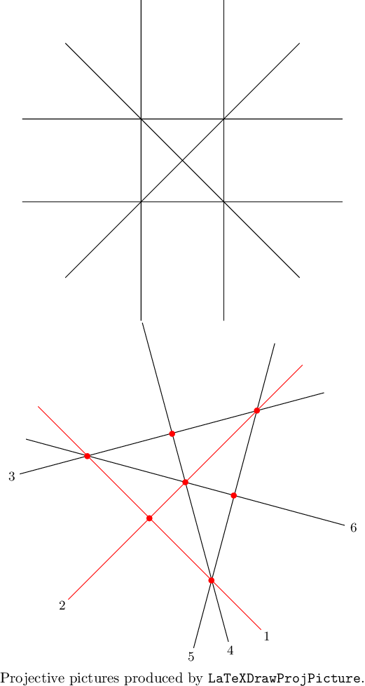
Generates LaTeX tikz-code for a nice projective picture of the real 3-arrangement. If x,y,z are the coordinates, by default, this is the 2-dim affine arrangement obtained by intersecting A with the plane z=1.
In the optional parameters DrawOptions, a record, the following parameters can be chosen
scale, a positive rational scaling factor,
isecps intersection points are drawn, true or false,
Hind labels for the hyperplanes are added, true or false,
deconeH a vector giving the normal of the plane (=1) with which to intersect A,
MarkHs a list of indices of hyperplanes of A, these are drawn in another color.
gap> A:=AGpql(2,2,3);
<HyperplaneArrangement: 6 hyperplanes in 3-space>
gap> Print(LaTeXDrawProjPicture(A));
\begin{tikzpicture}[scale=1.0]
\draw (-2.83,2.83) -- (2.83,-2.83);  % H_1
\draw (2.83,2.83) -- (-2.83,-2.83);  % H_2
\draw (-1.,3.87) -- (-1.,-3.87);  % H_3
\draw (1.,3.87) -- (1.,-3.87);  % H_4
\draw (3.87,-1.) -- (-3.87,-1.);  % H_5
\draw (3.87,1.) -- (-3.87,1.);  % H_6
\end{tikzpicture}
gap> DrawOpts:=rec(scale:=1/2,isecps:=true,Hind:=true,
>       deconeH:=[1,1,1],MarkHs:=[1,2]);;
gap> Print(LaTeXDrawProjPicture(AGpql(2,2,3),DrawOpts));
\begin{tikzpicture}[scale=1.0]
\draw[color=red] (-3.56,1.83) -- (1.83,-3.56);  % H_1
\node at (1.97,-3.71) {\small $1$};
\draw[color=red] (2.83,2.83) -- (-2.83,-2.83);  % H_2
\node at (-2.97,-2.97) {\small $2$};
\draw (3.35,2.16) -- (-4.,0.20);  % H_3
\node at (-4.20,0.14) {\small $3$};
\draw (-1.04,3.85) -- (1.04,-3.85);  % H_4
\node at (1.09,-4.06) {\small $4$};
\draw (2.16,3.35) -- (0.20,-4.);  % H_5
\node at (0.14,-4.20) {\small $5$};
\draw (-3.85,1.04) -- (3.85,-1.04);  % H_6
\node at (4.06,-1.09) {\small $6$};

\fill[red] (-0.87,-0.87) circle[radius=2pt];  % P[ 1, 2 ]
\fill[red] (-2.37,0.63) circle[radius=2pt];  % P[ 1, 3, 6 ]
\fill[red] (1.73,1.73) circle[radius=2pt];  % P[ 2, 3, 5 ]
\fill[red] (0.63,-2.37) circle[radius=2pt];  % P[ 1, 4, 5 ]
\fill[red] (0.0,0.0) circle[radius=2pt];  % P[ 2, 4, 6 ]
\fill[red] (-0.32,1.17) circle[radius=2pt];  % P[ 3, 4 ]
\fill[red] (1.17,-0.32) circle[radius=2pt];  % P[ 5, 6 ]
\end{tikzpicture}
The preceding example will look as follows
‣ LaTeXDrawSpherePicture( A ) | ( function ) |
Returns: A string.
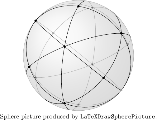
Generates LaTeX tikz-code for the intersection of a real 3-arrangement with the unit sphere. To compile the LaTeX-code the .sty-file "graphonsphere.sty" (from /doc/LaTeX_Examples) needs to be in the same folder and added via "\usepackage{graphonsphere}".
gap> A:=AGpql(2,2,3);
<HyperplaneArrangement: 6 hyperplanes in 3-space>
gap> Print(LaTeXDrawSpherePicture(A));
\tdplotsetmaincoords{63}{63}
\begin{tikzpicture}[scale=3,tdplot_main_coords]

\draw[ball color = gray!40, opacity = 0.2] (0,0,0) circle (1cm);

\def\OMcolor{black}
{\color{\OMcolor}
% the vertices of the OM-cpx
\foreach \i/\vx/\vy/\vz in {
1/0./0./1.,
2/-0.57/0.57/0.57,
3/-0.57/-0.57/0.57,
4/0.57/-0.57/0.57,
5/0.57/0.57/0.57,
6/0./1./0.,
7/1./0./0.,
8/0./0./-1.,
9/0.57/-0.57/-0.57,
10/0.57/0.57/-0.57,
11/-0.57/0.57/-0.57,
12/-0.57/-0.57/-0.57,
13/0./-1./0.,
14/-1./0./0.
}{
\node (\i) at (\vx,\vy,\vz) {};
\POnSfb{\vx}{\vy}{\vz}{}
}
%
% the edges of the OM-cpx
\foreach \ax/\ay/\az/\bx/\by/\bz in {
0./0./1./  -0.57/0.57/0.57, %[ 1, 2 ]
0./0./1./  -0.57/-0.57/0.57, %[ 1, 3 ]
0./0./1./  0.57/-0.57/0.57, %[ 1, 4 ]
0./0./1./  0.57/0.57/0.57, %[ 1, 5 ]
-0.57/0.57/0.57/  -0.57/-0.57/0.57, %[ 2, 3 ]
-0.57/0.57/0.57/  0.57/0.57/0.57, %[ 2, 5 ]
-0.57/0.57/0.57/  0./1./0., %[ 2, 6 ]
-0.57/0.57/0.57/  -0.57/0.57/-0.57, %[ 2, 11 ]
-0.57/0.57/0.57/  -1./0./0., %[ 2, 14 ]
-0.57/-0.57/0.57/  0.57/-0.57/0.57, %[ 3, 4 ]
-0.57/-0.57/0.57/  -0.57/-0.57/-0.57, %[ 3, 12 ]
-0.57/-0.57/0.57/  0./-1./0., %[ 3, 13 ]
-0.57/-0.57/0.57/  -1./0./0., %[ 3, 14 ]
0.57/-0.57/0.57/  0.57/0.57/0.57, %[ 4, 5 ]
0.57/-0.57/0.57/  1./0./0., %[ 4, 7 ]
0.57/-0.57/0.57/  0.57/-0.57/-0.57, %[ 4, 9 ]
0.57/-0.57/0.57/  0./-1./0., %[ 4, 13 ]
0.57/0.57/0.57/  0./1./0., %[ 5, 6 ]
0.57/0.57/0.57/  1./0./0., %[ 5, 7 ]
0.57/0.57/0.57/  0.57/0.57/-0.57, %[ 5, 10 ]
0./1./0./  0.57/0.57/-0.57, %[ 6, 10 ]
0./1./0./  -0.57/0.57/-0.57, %[ 6, 11 ]
1./0./0./  0.57/-0.57/-0.57, %[ 7, 9 ]
1./0./0./  0.57/0.57/-0.57, %[ 7, 10 ]
0./0./-1./  0.57/-0.57/-0.57, %[ 8, 9 ]
0./0./-1./  0.57/0.57/-0.57, %[ 8, 10 ]
0./0./-1./  -0.57/0.57/-0.57, %[ 8, 11 ]
0./0./-1./  -0.57/-0.57/-0.57, %[ 8, 12 ]
0.57/-0.57/-0.57/  0.57/0.57/-0.57, %[ 9, 10 ]
0.57/-0.57/-0.57/  -0.57/-0.57/-0.57, %[ 9, 12 ]
0.57/-0.57/-0.57/  0./-1./0., %[ 9, 13 ]
0.57/0.57/-0.57/  -0.57/0.57/-0.57, %[ 10, 11 ]
-0.57/0.57/-0.57/  -0.57/-0.57/-0.57, %[ 11, 12 ]
-0.57/0.57/-0.57/  -1./0./0., %[ 11, 14 ]
-0.57/-0.57/-0.57/  0./-1./0., %[ 12, 13 ]
-0.57/-0.57/-0.57/  -1./0./0. %[ 12, 14 ]
}{
\GCArcABfb{\ax}{\ay}{\az}{\bx}{\by}{\bz}{color=\OMcolor}
}
}
\end{tikzpicture}
The preceding example will look as follows
‣ LaTeXDrawTopeGraph( A ) | ( function ) |
Returns: A string.
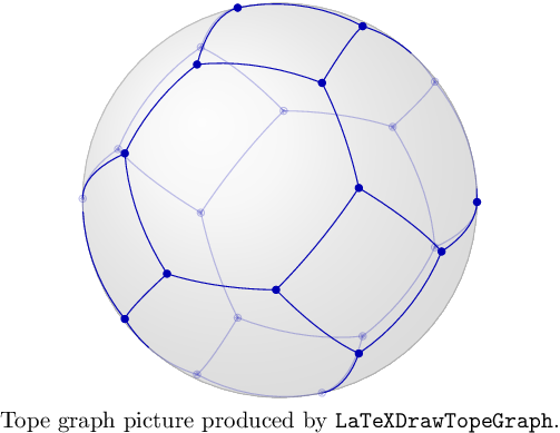
Generates LaTeX tikz-code for the tope graph of a real 3-arrangement on the unit sphere. To compile the LaTeX-code the .sty-file "graphonsphere.sty" (from /doc/LaTeX_Examples) needs to be in the same folder and added via "\usepackage{graphonsphere}".
gap> A:=AGpql(2,2,3);
<HyperplaneArrangement: 6 hyperplanes in 3-space>
gap> Print(LaTeXDrawTopeGraph(A));
\tdplotsetmaincoords{63}{63}
\begin{tikzpicture}[scale=3,tdplot_main_coords]
\draw[ball color = gray!40, opacity = 0.2] (0,0,0) circle (1cm);
\def\OMcolor{blue!70!black}
{\color{\OMcolor}
% the vertices of the OM-cpx
\foreach \i/\vx/\vy/\vz in {
1/-0.88/-0.47/0.,
2/0.88/0.47/0.,
3/-0.88/0./-0.47,
4/0.88/0./0.47,
5/-0.88/0./0.47,
6/0.88/0./-0.47,
7/-0.88/0.47/0.,
8/0.88/-0.47/0.,
9/-0.47/0./-0.88,
10/0.47/0./0.88,
11/-0.47/0./0.88,
12/0.47/0./-0.88,
13/-0.47/-0.88/0.,
14/0.47/0.88/0.,
15/0./-0.47/-0.88,
16/0./0.47/0.88,
17/0./-0.47/0.88,
18/0./0.47/-0.88,
19/0./-0.88/-0.47,
20/0./0.88/0.47,
21/0./-0.88/0.47,
22/0./0.88/-0.47,
23/0.47/-0.88/0.,
24/-0.47/0.88/0.
}{
\node (\i) at (\vx,\vy,\vz) {};
\POnSfb{\vx}{\vy}{\vz}{}
}
%
% the edges of the OM-cpx
\foreach \ax/\ay/\az/\bx/\by/\bz in {
-0.88/-0.47/0./  -0.88/0./-0.47, %[ 1, 3 ]
-0.88/-0.47/0./  -0.88/0./0.47, %[ 1, 5 ]
-0.88/-0.47/0./  -0.47/-0.88/0., %[ 1, 13 ]
0.88/0.47/0./  0.88/0./0.47, %[ 2, 4 ]
0.88/0.47/0./  0.88/0./-0.47, %[ 2, 6 ]
0.88/0.47/0./  0.47/0.88/0., %[ 2, 14 ]
-0.88/0./-0.47/  -0.88/0.47/0., %[ 3, 7 ]
-0.88/0./-0.47/  -0.47/0./-0.88, %[ 3, 9 ]
0.88/0./0.47/  0.88/-0.47/0., %[ 4, 8 ]
0.88/0./0.47/  0.47/0./0.88, %[ 4, 10 ]
-0.88/0./0.47/  -0.88/0.47/0., %[ 5, 7 ]
-0.88/0./0.47/  -0.47/0./0.88, %[ 5, 11 ]
0.88/0./-0.47/  0.88/-0.47/0., %[ 6, 8 ]
0.88/0./-0.47/  0.47/0./-0.88, %[ 6, 12 ]
-0.88/0.47/0./  -0.47/0.88/0., %[ 7, 24 ]
0.88/-0.47/0./  0.47/-0.88/0., %[ 8, 23 ]
-0.47/0./-0.88/  0./-0.47/-0.88, %[ 9, 15 ]
-0.47/0./-0.88/  0./0.47/-0.88, %[ 9, 18 ]
0.47/0./0.88/  0./0.47/0.88, %[ 10, 16 ]
0.47/0./0.88/  0./-0.47/0.88, %[ 10, 17 ]
-0.47/0./0.88/  0./0.47/0.88, %[ 11, 16 ]
-0.47/0./0.88/  0./-0.47/0.88, %[ 11, 17 ]
0.47/0./-0.88/  0./-0.47/-0.88, %[ 12, 15 ]
0.47/0./-0.88/  0./0.47/-0.88, %[ 12, 18 ]
-0.47/-0.88/0./  0./-0.88/-0.47, %[ 13, 19 ]
-0.47/-0.88/0./  0./-0.88/0.47, %[ 13, 21 ]
0.47/0.88/0./  0./0.88/0.47, %[ 14, 20 ]
0.47/0.88/0./  0./0.88/-0.47, %[ 14, 22 ]
0./-0.47/-0.88/  0./-0.88/-0.47, %[ 15, 19 ]
0./0.47/0.88/  0./0.88/0.47, %[ 16, 20 ]
0./-0.47/0.88/  0./-0.88/0.47, %[ 17, 21 ]
0./0.47/-0.88/  0./0.88/-0.47, %[ 18, 22 ]
0./-0.88/-0.47/  0.47/-0.88/0., %[ 19, 23 ]
0./0.88/0.47/  -0.47/0.88/0., %[ 20, 24 ]
0./-0.88/0.47/  0.47/-0.88/0., %[ 21, 23 ]
0./0.88/-0.47/  -0.47/0.88/0. %[ 22, 24 ]
}{
\GCArcABfb{\ax}{\ay}{\az}{\bx}{\by}{\bz}{color=\OMcolor}
}
}
\end{tikzpicture}
The preceding example will look as follows
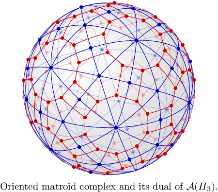
Both functions LaTexDrawSpherePicture and LaTeXDrawTopeGraph combined can be used to draw nice pictures of oriented matroid complexes and their duals.
generated by GAPDoc2HTML